The Bias-Variance Decomposition

The expected squared error of an estimator can be decomposed into a bias and a variance term. In order for the error to be minimal, generally not both, bias and variance, can be minimal. This is the bias-variance trade-off.

The data

Consider a dataset

with inputs \(x\) and targets \(y\). Assume that the targets are generated by the relation

where \(f(x)\) is a deterministic, but unknown map.

The scalar \(\epsilon\sim p(\epsilon)\) is an additive noise term with zero mean \(\operatorname{Exp}[\epsilon]=0\) and finite variance \(\operatorname{Var}[\epsilon]=\sigma^2\). More generally, we can assume some data-generating process \((x, y)\sim p(x, y)\) that is obeying Eq. \eqref{eq:y}, and by extension a distribution over datasets of size \(N\)

one realization of which is the dataset at hand (\(\mathcal{D}\) hence denotes both, the given dataset and the random variable).

The estimator

Since the relation \(f\) in Eq. \eqref{eq:y} is unknown, we would like to estimate it from the given dataset \(\mathcal{D}\).

Hence, consider a model \(\hat{f}_{\mathcal{D}}\) that is fitted to \(\mathcal{D}\) and can produce a prediction \(\hat{f}_{\mathcal{D}}(x)\) for some given \(x\), where \(x\) is not necessarily in the dataset. This prediction estimates (guesses, based on data and model assumptions) the unknown value \(f(x)\). The function \(f_{\mathcal{D}}(x)\) is called an estimator for \(f(x)\).

Further, if we take Eq. \eqref{eq:D} seriously and assume that \(\mathcal{D}\) is a random variable, by extension, the estimator \(\hat{f}_{\mathcal{D}}(x)\) is a random variable, too.

What is the bias of an estimator?

The bias of the estimator \(\hat{f}_{\mathcal{D}}(x)\) is defined as the difference between its expectation w.r.t. \(p(\mathcal{D})\) and the ground truth value \(f(x)\)

The bias thus tells us how much the prediction \(\hat{f}_{\mathcal{D}}(x)\) deviates from the true value \(f(x)\) on average, where the average is taken over all potential datasets \(\mathcal{D}\) weighted with the probability they occur. If the bias is zero, it means that the model on average yields the correct prediction. Keep in mind tough, that the bias is a theoretical construct involving the ground truth \(f(x)\) and is generally not tractable.

While the bias tells us about the goodness of the average prediction, it does not tell us how predictions \(\hat{f}_{\mathcal{D}}(x)\) for individual datasets may differ from one another. This is encoded in the variance of \(\hat{f}_{\mathcal{D}}(x)\) which we discuss next.

What is the variance of an estimator?

Again assume all the above, and especially \(\mathcal{D}\sim p(\mathcal{D})\). The variance of the estimator \(\hat{f}_{\mathcal{D}}(x)\) is defined as

Hence, the variance is the expected square deviation of the estimator from its mean. While the bias of \(\hat{f}_{\mathcal{D}}(x)\) depends on the ground truth \(f(x)\), the variance does not; it simply quantifies the spread of the individual estimators. However, like the bias, the variance is usually not tractable either since the expectation over \(p(\mathcal{D})\) cannot be computed.

The bias-variance decomposition of the expected squared error

The bias and variance each describe one aspect of the estimator \(\hat{f}_{\mathcal{D}}(x)\) and each individually give an incomplete picture of its behavior. But, do they give a complete picture together? The answer is generally no, but there is one interesting exception:

Assuming the data-generation as above, the expected squared error of the estimator \(\hat{f}_{\mathcal{D}}(x)\) can be decomposed into its bias squared, its variance and an independent, irreducible error that depends on the observation noise \(\epsilon\).

Consider the squared error (square loss)

as a measure for the performance of \(\hat{f}_{\mathcal{D}}(x)\) on the pair \((x, y)\). The highlighted statement above means that the expected squared error can be decomposed as follows:

where \(\sigma^2=\operatorname{Var}[\epsilon]\) is the irreducible error. This is the bias-variance decomposition of the expected squared error.

The derivation is straightforward and can be done by expanding terms and applying the expectation where possible.

The bias-variance trade-off

The expected squared error, as well as all summands in the second line of Eq. \eqref{eq:decomp} are non-negative. The usual intuition is that, when varying the estimator \(\hat{f}_{\mathcal{D}}(x)\), if its squared bias gets smaller, its variance gets larger and vice versa. This means that there is an optimal \(\hat{f}^*_{\mathcal{D}}(x)\) where the expected squared error, but generally neither the squared bias, nor variance is minimal. This is the bias-variance trade-off. In formulas, if

then in general

Varying the estimator here may mean to use a different model for \(\hat{f}_{\mathcal{D}}\) or a different fitting procedure, or more generally to vary the deterministic mechanism that retrieves \(\hat{f}_{\mathcal{D}}\) from \(\mathcal{D}\). The irreducible error \(\sigma^2\) does not play a role as it is a constant w.r.t. \(\hat{f}_{\mathcal{D}}\).

The above (in)equalities suggest that, at least under the square loss (and possibly elsewhere, too), a non-zero bias of an estimator is not a bad thing if one is interested in its predictive performance.

Illustrative example

The bias-variance trade-off is often explained with the expressiveness of the model \(\hat{f}_{\mathcal{D}}\) and its flexibility to fit the data. For instance, a simple model such as linear regression with a small amount of features may yield similar predictions no matter the dataset \(\mathcal{D}\) in which case its variance is low, but its bias is large as it never can fully express the ground truth \(f(x)\). An expressive model on the other hand—let’s say linear regression with many features—may be able to represent \(f(x)\) and even “patterns” in \(\mathcal{D}\) that are due to the noise term \(\epsilon\). In this case, the bias may be low, but the variance may be high. The latter is often associated with “overfitting” (model is too flexible with the data) and the former with “underfitting” (model is too rigid), although underfitting is a less well-defined term.

As an illustrative example, consider the function

where \(\Phi(x) = [1, \sin(x), \cos(x), \sin(2x), \cos(2x), \dots, \sin(Kx), \cos(Kx)]\in\mathbb{R}^{2K+1}\) are some Fourier features and \(w=[w_1, w_2, \dots, w_{2K+1}]\in\mathbb{R}^{2K+1}\) are some fixed parameters.

The ground truth function

As ground truth function, we use \(K=3\), that is \(f(x):=g(x, K=3)\) and some fixed parameters \(w\).

import numpy as np

def _features_fourier(x, K):
    """Computes K Fourier features for x."""
    features = np.zeros([x.shape[0], int(1 + 2 * K)])
    for i, xi in enumerate(x):
        features_i = [1.0]        
        for k in range(1, K+1):
            features_i = features_i + [np.sin(k * xi), np.cos(k*xi)]
        features[i, :] = np.array(features_i)
    return features


def f(x):
    """The ground truth function."""
    # Fourier features for K=3
    ff = _features_fourier(x, 3)
    # 2*K + 1 fixed parameters w
    w = np.array([ 0.49671415, -0.1382643 ,  0.64768854,  1.52302986, -0.23415337, -0.23413696,  1.57921282])
    return ff @ w

The resulting ground truth function \(f(x)\) is plotted below on the x-range \([0, 10]\).

The data

We know the data must obey Eq. \eqref{eq:y} with an \(\epsilon\) that has zero mean and finite variance \(\operatorname{Var}[\epsilon]=\sigma^2\). Hence, we choose to produce each dataset according to:

def sample_dataset(N, sigma):
    X = np.random.uniform(0, 10, N)
    F = f(X)
    Y = F + sigma * np.random.randn(N)
    return X, Y, F

N = 50
sigma = 0.8
X, Y, F = sample_dataset(N, sigma)

Each dataset is of size \(N=50\) in this example. Since we want to illustrate the intractable bias of an estimator we also return the unperturbed ground truth values \(f(x)\) (stored in the array F) which we would not know in practice. Similarly, \(\sigma\) may or may not be known in practice. One example of a dataset is plotted below (blue dots scattered) with the ground truth function as dotted line. The datapoints do not exactly lie on top of the function due to the noise term \(\epsilon\). A good estimator should avoid fitting those “wiggles” and rather smooth them out to fit the dotted line more closely.

Further, we denote the set of nodes, observations and ground truth values as \(X=[x_1,\dots,x_N]\in\mathbb{R}^{N}\), \(Y=[y_1,\dots,y_N]\in\mathbb{R}^{N}\) and \(F=[f(x_1),\dots,f(x_N)]\in\mathbb{R}^{N}\) respectively. The feature matrix is denoted as \(\Phi(X)\in\mathbb{R}^{N\times (2K + 1)}\) where \([\Phi(X)]_{ik} = \Phi_k(x_i)\) with \(i=1,\dots,N\) and \(k=1,\dots, (2K+1)\).

Estimators with increasing complexity

For our illustrative purposes we create 14 estimators with increasing complexity that have the functional form as in Eq. \eqref{eq:g} with \(K\) ranging from 0 to 13. The estimators are then fitted to the data via least squares. That is, the \(w\) parameters are the minimizers of the empirical square loss

which admits an analytic solution \(\hat{w} = [\Phi(X)^{\intercal}\Phi(X)]^{-1}\Phi(X)^{\intercal}Y\). To make the dependence on \(K\) explicit, we write

This means, our 13 estimators are the functions \(\hat{f}_{\mathcal{D}}(x, K=0), \hat{f}_{\mathcal{D}}(x, K=1),\dots,\hat{f}_{\mathcal{D}}(x, K=13)\) with increasing complexity.

def _solve_linear_least_squares(features, Y):
    return np.linalg.lstsq(features, Y)

def compute_weights(X, Y, Phi):
    features = Phi(X)
    gram = features.T @ features
    b = features.T @ Y
    return _solve_linear_least_squares(gram, b)[0]

def fhat_from_weights(x_test, w, Phi):
    features = Phi(x_test)
    return features @ w    

# Example of fitting the estimator with K = 5 to the data X, Y
K = 5
Phi = lambda x: _features_fourier(x, K)
w_hat = compute_weights(X, Y, Phi)
fhat = lambda x: fhat_from_weights(x, w_hat, Phi)

# evaluate on random test point
x_test = np.atleast_1d(np.random.uniform(0, 10, 1))
f_hat_at_x_test = fhat(x_test)

Estimation of bias and variance

Recall that the bias and the variance of an estimator are generally not tractable. For each of the 14 estimators, we thus approximate those two quantities by computing the expectations over \(p(\mathcal{D})\) with Monte Carlo using \(10^3\) samples. This means, for each estimator, we draw \(10^3\) datasets of size \(N=50\), we fit the estimator to each dataset with Eq. \eqref{eq:fhat}. This yields \(10^3\) predictions on a test point which we choose randomly to be \(x\approx 8.96\). The results are then used to approximate the expectations required to compute the bias and the variance term.

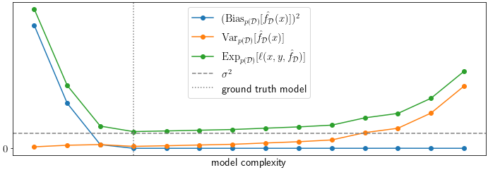
The plot below shows the squared bias, the variance, the expected loss and \(\sigma^2\) versus \(K\) of the estimators which is a proxy for the model complexity. The “ground truth model”, meaning the estimator which uses the same \(K\) as the ground truth function \(f\) is marked with a vertical dotted line at \(K=3\). Unsurprisingly, it also happens to be the best estimator as it exhibits the minimal expected error on the test point. As expected, neither its variance, nor its squared bias is minimal when compared to all other estimators.

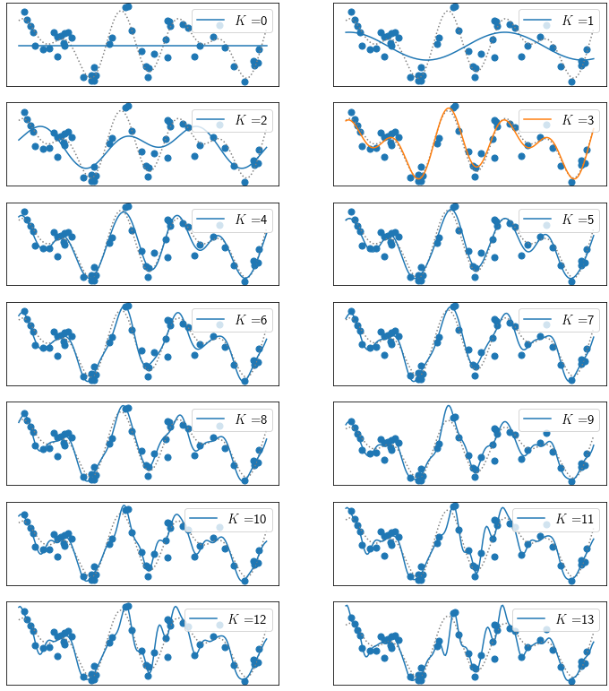
The behavior of the estimators can be understood by looking at individual fits. The following plots shows fits of all 14 estimators to one of the datasets of size \(N=50\). The estimator with minimal expected squared error (with \(K=3\)) is shown in orange. It is apparent that less complex estimators with a lower \(K\) are too rigid to fit the underlying function well which explains the large bias and low variance term, while the more complex models even fit to the noise term \(\epsilon\) which explains their large variance. The winning model with \(K=3\) has just the right complexity to explain the signal, but smooth out the perturbations \(\epsilon\).

It should be noted that the intuition presented here may not be applicable to all estimators out there, especially if the model is a poor representation of the ground truth, no matter its complexity. Additionally, there may be other effects at play that are less well understood. For instance, there is some empirical evidence in deep learning that heavily over-parameterized deep networks, which are very flexible estimators, may still yield a meaningful bias-variance trade-off (e.g., [1]).

References

[1] Nakkiran et al. 2020 Deep Double Descent: Where Bigger Models and More Data Hurt, ICLR.