Invariant Gaussian Processes

Gaussian processes can be understood as “distributions over functions” providing prior models for unknown functions. The kernel which identifies the GP can be used to encode known properties of the function such as smoothness or stationarity. A somewhat more exotic characteristic is invariance to input transformations which we’ll explore here.

What is an invariant function?

I came across the paper of Wilk et al. 2018 a while ago which introduces Gaussian processes that are invariant under a finite set of input transformations. Let’s first see what an invariant function is: A function \(f:\mathcal{X} \rightarrow \mathbb{R}\) on the domain \(\mathcal{X}\subseteq\mathbb{R}^D\) is said to be invariant under a bijective transformation \(T:\mathcal{X}\rightarrow \mathcal{X}\) if \(f(T(x)) = f(x)\) holds for all \(x\) in \(\mathcal{X}\). This simply means that the function \(f\) takes the same value at \(x\) and \(T(x)\) for all \(x\).

Simple 1D example: \(f(x) = x^2\) is invariant under flipping the x-axis, i.e., \(f(x) = f(-x)\) with \(T(x) = -x\), and \(x\in\mathbb{R}\).

Invariance groups and orbits

Consider now a function that is invariant under a finite set of \(J\) transformations \(T_i\), \(i=1, ..., J\). As the invariance under each \(T_i\) holds for any input \(x\) (also those that have been transformed), the \(T_i\) must form the group \(G_f:=\{T | f(x) = f(T(x)) \text{ for all } x \in\mathcal{X}\}\). That is, \(G_f\) contains arbitrary concatenations \(T_i\circ T_j\circ \dots\), the identity transform \(T=I\), the inverses \(T_i^{-1}\), and the \(T_i\) obey associativity. There may be several groups associated with a function \(f\), depending on which invariances are considered.

For the above example \(f(x) = x^2\), the implied group \(G_f\) only contains \(J=2\) transformations \(G_f = \{T_0, T_1\}\) with \(T_0(x)=x\) and \(T_1(x)=-x\). This is because all possible concatenations \(T_i\circ T_j\circ \dots\) as well as the inverses \(T_i^{-1}\) collapse back to \(T_0\) or \(T_1\) and are thus already in \(G_f\) (Examples: \(T_1^{-1} = T_1\), or \(T_1\circ (T_1 \circ T_1) = T_1\circ T_0 = T_1\) etc).

Given \(G_f\), the set \(\mathcal{A}(x):=\{T(x) | \text{ for all } T\in G_f\}\) is called an orbit of \(x\) and is the set of invariant locations induced by \(x\).

In our 1D example \(f(x) = x^2\) with \(G_f\) containing \(T_0\) and \(T_1\), consider an arbitrary point e.g., \(x^* = 0.2\). The orbit of \(x^*\) is then given by \(\mathcal{A}(x^*) = \{T_0(x^*), T_1(x^*)\} = \{0.2, -0.2\}\).

Modelling an invariant black-box function

Given \(G_f\) and \(\mathcal{A}(x)\), we can now introduce a latent function \(g: \mathcal{X} \rightarrow \mathbb{R}\) such that

The latent function \(g\) is not necessarily invariant, but the function \(f\) is by construction. This is because any point \(\tilde{x}\in \mathcal{A}(x)\) induces the identical set \(\mathcal{A}(\tilde{x}) = \mathcal{A}(x)\), hence \(f(\tilde{x}) = f(x)\) for all \(\tilde{x}\in A(x)\). (notice that \(G_f\) includes the identity transform, the trivial invariance for all functions).

We see from the above equation that we do not need to know the form of \(f(x)\) in order to encode the invariance property, simple knowing the set \(G_f\) is enough. In that sense, \(f(x)\) can be a black-box function.

Making it probabilistic (An invariant Gaussian process prior)

If the function \(f\) is unknown, and we want to learn it from a set of function evaluations, we can treat the inference problem probabilistically to account for the uncertainty of value of \(f\) where \(f(x)\) is not observed. In certain circumstance, a good choice of models are Gaussian processes (GPs), especially since they let us encode properties of the function leading to sample efficient learning methods. In our case, the property we want to encode is the invariance of \(f\) under the group \(G_f\) as defined above. We again follow Wilk et al. 2018 (Section 4.1).

In essence, the trick is to model the latent function \(g\) as a Gaussian process \(g\sim\mathcal{G}(m_g, k_g)\) with mean function \(m_g\) and kernel function \(k_g\) such that the resulting process on \(f\) obeys the invariance by the above construction. It turns out that then, \(f\) is also a Gaussian process \(f\sim\mathcal{G}(m_f, k_f)\), as \(f\) is a linear combination (weighted sum) of jointly Gaussian distributed values \(g\) (and Gaussians are closed under linear transformations). The mean function \(m_f\) and kernel function \(k_f\) can be easily derived:

GP regression on \(f\) is straightforward, too, as the above equation simply defines another positive definite kernel \(k_f\). In essence, we did not transform the distribution of \(g\) itself, we merely correlated function values of \(g\) at invariant locations in input space.

Pretty Priors: Samples of invariant GPs

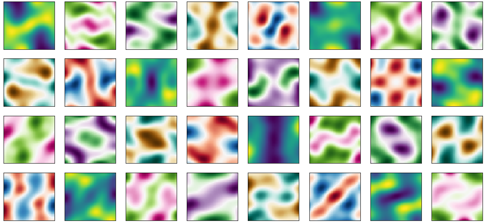
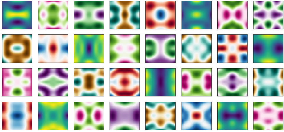
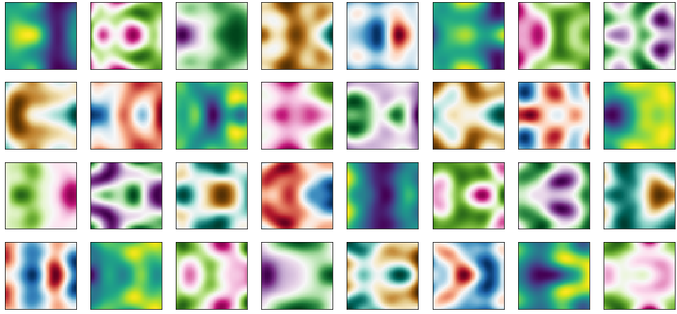
Let’s create some plots. Below we plot 4 x 8 = 32 samples of invariant Gaussian processes with a 2D input domain. The samples are from the prior GP not conditions on any data. We can see that the samples obey the invariances encoded. This means that the model, if conditioned on function evaluation, needs not learn the invariance property of the function from the data, as it is already encoded in the prior. This will likely lead to sample-efficient algorithms.

Point-symmetry

Group \(G_f\) is of size \(J=2\) and contains \(T_0= I\) as well as a projection operator though the origin (flipping all signs) \(T_1 = -1\). This encodes point-symmetry of \(f\) through the origin as can be seen from the prior samples (the origin at \([0, 0]\) is in the center of each plot).

Axis-symmetry along both axis

In order to encode axis-symmetry along both axis, we need to add two additional invariances \(T_2\) and \(T_3\) in addition to \(T_0\) and \(T_1\) above (total of \(J=4\) transformations). \(T_2\) and \(T_3\) each flip the sign of one axis, that is \(T_3 = [[-1, 0]; [0, 1]]\) and \(T_3 = [[1, 0]; [0, -1]]\). We observe that the samples from this prior observe the axis-symmetries.

Axis-symmetry along one axis

For axis-symmetry along one axis only (say x-axis), we only require \(J=2\) transformations given by \(T_0=I\) and \(T_1 = [[1, 0]; [0, -1]]\). The samples again obey the symmetry.

Rotations

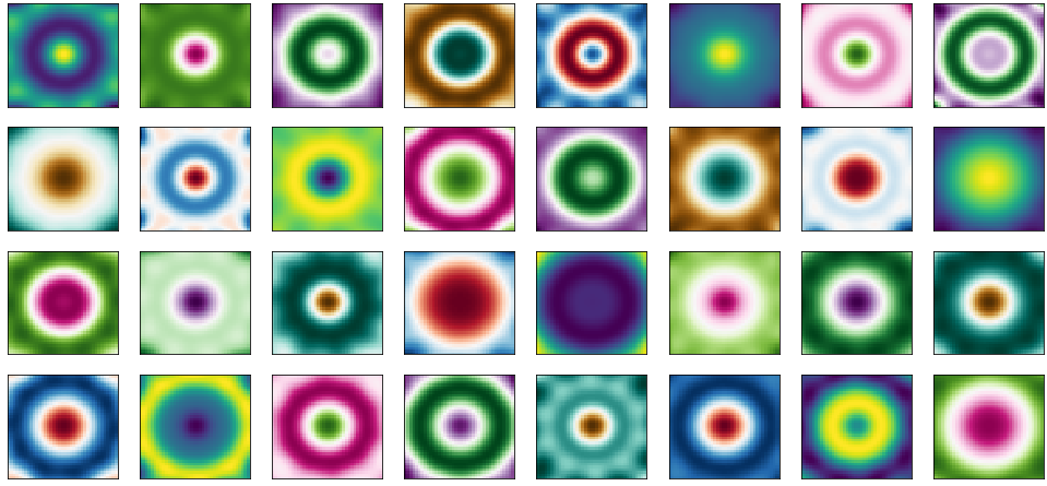
Lastly, for \(J\)-fold rotational symmetry, the group \(G_f\) contains \(J\)-fold rotation matrices with \(T_i = R(\theta=i\frac{2\pi}{J})\) for \(i=1,\dots,J\) where \(R(\theta)\) is the 2D rotation matrix. Below we show \(J=5\).

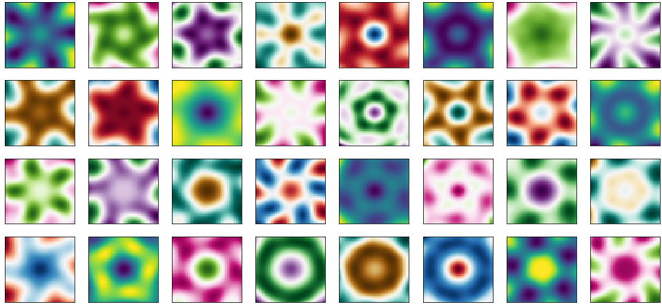
Same as above but for \(10\)-fold rotation (\(J=10\)).

Where is the data?

Nowhere yet. I may write another blogpost showing posterior samples from the invariant GPs. They look quite cool indeed, as the invariant GP seems to “learn” at locations where nothing is observed (this is at and close to points that are invariant to observed points under the model). I may also discuss algorithmic complexity there.

References

[1] Wilk et al. 2018 Learning invariances using the marginal likelihood, Advances in Neural Information Processing Systems 31, pages 9938–9948.

[2] Rasmussen and Williams 2006. Gaussian Processes for Machine Learning. Adaptive Computation and Machine Learning. MIT Press, Cambridge, MA, USA.