The Standard Error

The law of large numbers (previous post) can be combined with the standard error (SE) in order to not only get an estimate of a parameter, but also a notion of the robustness of said estimate. Thus, the standard error lets us know how confident we can be about our estimation.

In the previous post, we learned that, by the law of large numbers (LLN), the sample mean \(\bar{x}_n\) tends to the population mean \(\mu\) in some sense for large enough \(n\) (see previous post for notation). We have also empirically observed (for fair coin tosses with \(\mu=0.5\)) that the sample size \(n\) needs not be overly large (roughly \(> 100\)) in order to yield a somewhat relivable estimate of the coin-flip-parameter \(\mu\).

Similarly, we have observed that the statistic \(\bar{x}_n\) by definition is a random number, as it is the average of random coin tosses. For any finite \(n\) the statistic \(\bar{x}_n\) thus exhibits a certain variability which means that it’s value might be different if we repeat the experiment and toss the coin another \(n\) times (and then compute \(\bar{x}_n\) from the new coin tosses/ the new sample). The standard error \(\sigma_n\) quantifies this variability. In particular the SE has the following form

where \(\sigma := \operatorname{Std}[x]\) is the standard deviation of the random variable \(x\) that represents a single coin toss. It is apparent that the SE drops proportional to one over the squareroot of \(n\), that is \(SE[\bar{x}_n] \propto n^{-\frac{1}{2}}\). This behavior is called the squareroot law.

How wrong can it be? The most (?) important characteristic of the SE

In addition to the squareroot law, we observe that the SE is independent of the population size as it only depends on the population variance \(\sigma^2\) and the sample size \(n\). This is surprising but also very useful as it means that a low variability of the statistic \(\bar{x}_n\) for a large population can be achieved with a similar sample size as for a small population. As example, let’s consider two countries, one of them small, and one of them large in population, and (for the sake of argument) both currently having the same approval rate \(\mu\) of their presidents (in this particular example, this implies same \(\sigma\)). The SE formula now states that in order to obtain the same expected precision on the statistic \(\bar{x}_n\) representing the approval rate of each president, the survey conducted in the large country requires the identical (relatively small) sample size \(n\) as the survey conducted in the small country. In other words, each survey simply needs to select a few hundred to a few thousand random voters to obtain a statistic of good enough representative power, no matter the size of the country. There are of course practical limitations to consider (some are briefly mentioned below), but this astonishing characteristic of the SE holds in theory and has proven successful in practice as well. Let’s have a closer look at the SE formula now, and introduce some notation. Then, we’ll empirically observe the behavior of the SE on the example of coin tosses.

The Standard Error Formula

Let \(\zeta_1, \dots, \zeta_k\) be uncorrelated (not necessarily independent or identically distributed) random variables, that is \(\operatorname{Cov}[\zeta_j, \zeta_l] = 0\) if \(j\neq l\) and \(j, l=1,\dots, l\) with corresponding variances \(\sigma^2_{\zeta_j}:=\operatorname{Var}[\zeta_j]\), \(j=1,\dots, k\). Then, Bienaymé’s formula states that the variance of the sum \(S_k^{\zeta} :=\sum_{j=1}^k \zeta_j\) is equal to the sum of the variances of the \(\zeta\)s, that is \(\operatorname{Var}[S_k^{\zeta}] = \sum_{j=1}^k \sigma^2_{\zeta_j}\).

In our example, the single coin tosses \(x_i\) comprising the sample are uncorrelated as they are independent, and, as they are identically distributed, all have same variance \(\sigma^2\). Hence, the variance of their sum \(S_{n}^x:=\sum_{i=1}^n x_n\) is \(n\) times the variance of \(x\) that is \(\operatorname{Var}[S_n^x] = \sum_{i=1}^n \operatorname{Var}[x_i] = \sum_{i=1}^n \sigma^2 = n\sigma^2\). The SE of \(\bar{x}_n\) which is equal to its standard deviation is thus

which (equality of leftmost and rightmost term) is the formula stated above. We’ll illustrate the SE again with the example of fair coin tosses.

Tossing Coins Again

A single fair coin toss \(x\) follows a Bernoulli distribution with parameter \(\mu=0.5\). We know that Bernoulli random numbers have variance \(\sigma^2 = \mu(1-\mu)\). Hence, we can compute the statistic \(\bar{x}_n\) and the SE as \(SE[\bar{x}_n] = \frac{\sqrt{\mu(1-\mu)}}{\sqrt{n}} = \frac{0.5}{\sqrt{n}}\).

import numpy as np
np.random.seed(42)

# fair coin
mu = 0.5

# Bernoulli samples: 1 means heads, 0 means tails
n_samples = int(1e4)
samples = 1 * (np.random.rand(n_samples) < mu)

# Compute mean statistic and its standard error
S = np.cumsum(samples)
n =  np.arange(1, n_samples + 1)
means = S / n
standard_errors = np.sqrt(mu * (1 - mu)) / np.sqrt(n)

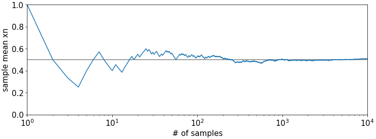
First we plot \(\bar{x}_n\) versus the number of samples \(n\) (blue solid). The horizontal gray line indicates the ground truth \(\mu=0.5\). We observe that \(\bar{x}_n\) approaches \(\mu\) for larger \(n\); this is due to the law of large numbers (LLN). The x-axis is in log-scale on all plots.

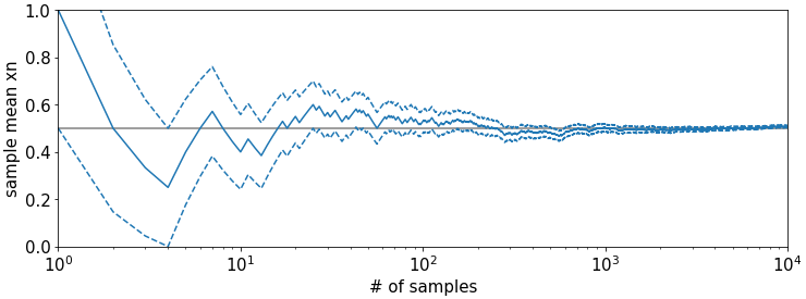
Now we plot both \(\bar{x}_n\) (solid blue) and the interval \(\bar{x}_n\pm \frac{0.5}{\sqrt{n}}\) (dashed blue). We observe that the area between the dashed lines most of the time (for most \(n\)) but not every time encloses the true parameter \(\mu\). We also observe that the interval shrinks the larger \(n\) according to the squareroot law.

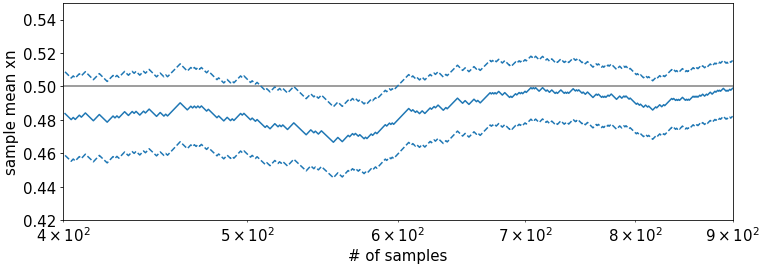
The plot below is a zoomed in version of the above plot for samples sizes between \(n=400,\dots,900\). It is better visible here that not all intervals enclose \(\mu\).

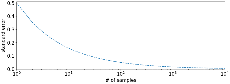
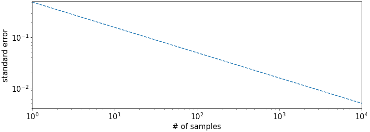
To illustrate the decay of the SE, we also plot the standalone \(SE[\bar{x}_n] = \frac{0.5}{\sqrt{n}}\) on a linear y-scale,

and on a logarithmic y-scale. In the logarithmic plot we can better observe the linear decay \(\log SE[\bar{x}_n] \propto -\frac{1}{2}\log n\) with slope \(-\frac{1}{2}\).

The Catch Again

Besides, requiring truly random numbers which (as mentioned in the previous post) are hard to obtain, the SE formula has two major drawbacks.

First, the decay rate of the SE \(n^{-\frac{1}{2}}\) is very slow. It means that e.g., 4 times the sample size will only half the standard error, 100 times the sample size will reduce the SE by 1/10th, and \(10^4\) times the sample size will only reduce the SE by a factor of 100 etc. It is apparent that the sample size required to obtain small SEs explodes pretty fast. Therefore, it is very hard to obtain high precision estimates with this method. The root cause of this is the underlying random sampling mechanism. However, for rough but still reliable estimates, the statistic \(\bar{x}_n\) together with its SE is an incredibly valuable tool. With some further assumptions on the form of \(p(\bar{x}_n)\) that are often justified in practice, one can even use the SE to obtain confidence intervals. But this is a topic for another post :)

Second, it requires us to know the population variance \(\sigma^2\) which in practice is usually not accessible (to compute it we would require access to the whole population which is precisely not what we want). In the example above, this did not matter as we had access to the ground truth values \(\sigma^2\) and \(\mu\). This is usually not the case. Generally, how this is handled is via the boostrap principle, where either i) \(\sigma^2\) is being estimated from the sample, or ii) the SE is being estimated via boostrap sampling. But this, too, is a topic for another post :)