The Tesseract

The tesseract is a 4-dimensional hyper-cube which is fun to animate by rotating it around one or more planes and projecting it onto 3-dimensional space. The post also contains animations of a rotating 4-dimensional sphere.

The analogue to the tesseract in 3d is the cube, and in 2d the square.

Tesseract construction & 4-dimensional vectors

We are in 4-dimensional space, hence denote \(d=4\). We can describe the tesseract with the coordinates of its corners. These are all \(2^d=16\) combinations of

for a tesseract centered at the origin. Hence, we can initialize our tesseract by storing these 16 corner vectors. Since it is custom to denote the axis of a vector in 3-dimensional space with the letters \(x\), \(y\), \(z\), we’ll extend the notation and use \(w\) for the forth axis.

4-dimensional plane rotations

In 2-dimensional space, we rotate around a point, in 3-dimensional space, we rotate around an axis, and in 4-dimensional space where the tesseract lives, we rotate around a plane.

In essence, a rotation is a circular movement in a plane that is spanned by 2 vectors, and the remaining space with dimensionality \(d-2\) stays invariant and is hence “rotated around”. In 4-dimensional space, there are 6 axis-aligned planes. These are the i) \(x\)-\(y\), ii) \(x\)-\(z\), iii) \(x\)-\(w\), iv) \(y\)-\(z\), v) \(y\)-\(w\), and vi) \(z\)-\(w\) plane.

For some angle \(\theta\), the corresponding axis-aligned \(d\times d\) rotation matrix \(R\) in Python code is given by

import numpy as np

# Choose 2 axis in which the circular movement occurs.
# The rotation plane is spanned by the remaining 2 axis.
a = 'x'
b = 'y'

# Choose angle
theta = 0.2

# Convert axis name to axis index
axis_dict = {'x': 0, 'y': 1, 'z': 2, 'w': 3}
i = axis_dict[a]
j = axis_dict[b]

# Build rotation matrix
R = np.eye(4)
R[i, i] = np.cos(theta)
R[j, j] = np.cos(theta)
R[i, j] = -np.sin(theta)
R[j, i] = np.sin(theta)

The axes \(a\) and \(b\) chosen in the code snippet above are the axis that the rotation (circular movement) is happening in. The remaining 2 axis stay invariant under this rotation and hence span the rotation plane. For example if \(a=x\) and \(b=y\), the rotation plane is the \(z\)-\(w\) plane.

Projection onto 3-dimensional space

To visualize the 4-dimensional tesseract, we require an at most 3-dimensional representation. There are several ways to project a higher-dimensional object onto a lower-dimensional space. A simple one is the stereographic projection where a point light source projects the shadow of a \(d\)-dimensional object onto a \(d-1\) dimensional “screen” (or rather hyper-screen). For the tesseract, the hyper-screen is usually chosen to be the space spanned by the \(x\), \(y\) and \(z\) axes’ unit vectors. Then, the \(d-1\) dimensional projected vectors \(\bar{v}\) have the form

where \(\delta\) is a positive scalar related to distance between the light-source and the hyper-screen. We can choose \(\delta\) arbitrarily, as long as the object we project still fits in between the light source and the hyper-screen (i.e., \(\delta\) must be large enough).

The stereographic projection is intuitive. We observe that the remaining elements of \(v\) in \(\bar{v}\) are multiplied with the scale \((\delta-v_w)^{-1}\). This scale is constant for each corner vector, but differs between vectors depending on the value of the \(v_w\). Hence, corners of the tesseract that are closer to the light source (larger \(v_w\)) and further away from the screen will be shown larger on the screen than corners that are closer to the screen and further away from the light source. In that way, the value of the 4th dimension \(v_w\) is implicitly represented in all elements of \(\bar{v}\).

Rotating tesseract

The following animations use the above projection. The tesseract is initialized as in Eq. \eqref{eq:init}.

From left to right (or top to bottom) the animations show i) rotation in \(x\)-\(y\) plane (\(z\)-\(w\) rotation plane stays invariant) ii) rotation in \(z\)-\(w\) plane, (\(x\)-\(y\) rotation plane stays invariant) iii) double rotation in \(x\)-\(y\) and \(z\)-\(w\) planes.

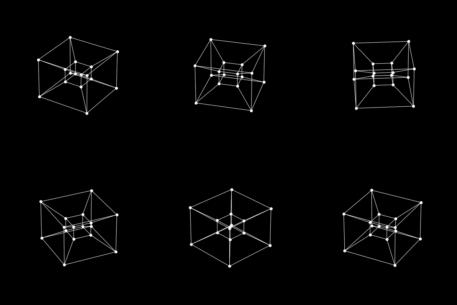
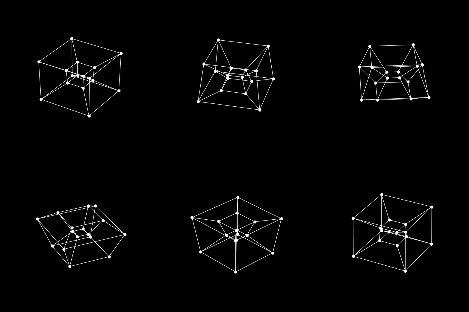
The corners only move “in” and “out” w.r.t. the origin when the rotation involves movement in the \(w\) axis. The 32 edges of the tesseract are drawn as lines in the animation.

Rotating 4-dimensional hyper-sphere

A 4-dimensional centered hyper-sphere is the collection of points for which \(v_x^2 + v_y^2 + v_z^2 + v_w^2 = r^2\), where \(r\) is the radius of the sphere.

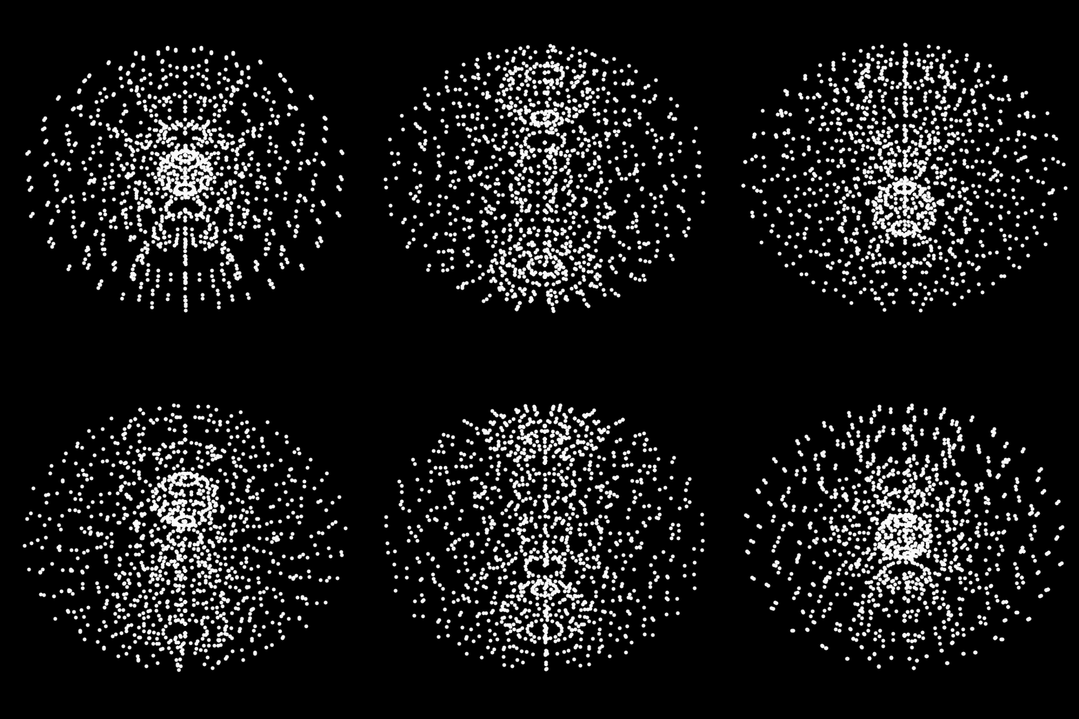
At first, it may sound boring to rotate and animate a centered sphere (shouldn’t it be symmetrical?). Since this is true, we represent the surface of the hyper-sphere with dots, each represented by a 4-dimensional vector, and observe their movement when rotated on the hyper-screen. The dots are spread according to:

import numpy as np

# Choose radius of sphere.
r = 1

# Grid of angles
z_ = np.linspace(0, 2 * np.pi, 20)
x_ = np.linspace(0, 1 * np.pi, 10)
y_ = np.linspace(0, 1 * np.pi, 10)
theta1, theta2, theta3 = np.meshgrid(x_, y_, z_, indexing='ij')

x = r * np.sin(theta1) * np.sin(theta2) * np.cos(theta3)
y = r * np.sin(theta1) * np.sin(theta2) * np.sin(theta3)
z = r * np.sin(theta1) * np.cos(theta2)
w = r * np.cos(theta1)

The above code snipped uses spherical coordinates in \(d=4\) dimensions that are given by the radius \(r\) and \(d-1\) angles \(\theta_1,\dots,\theta_{d-1}\) . In total, we distribute \(2000=10\times 10\times 20\) points on the surface of the hyper-sphere. The points are chosen ad-hoc and not spread uniformly.

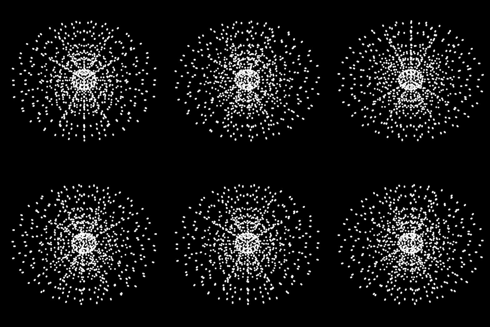
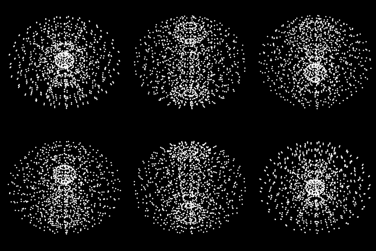
The animations below (from left to right or top to bottom) show the same rotations as the ones of the tesseract above. Whenever a rotation involves movement in the \(w\) axis, the dots representing the surface of the sphere move in, or outwards in the animation.

Some thoughts

The rotating tesseract and the hyper-sphere are simple enough to animate. In 4 dimensions all you need are some vectors and a rotation matrix. There are little things simpler to write in code than a matrix-vector multiplication which is effectively what this boils down to. The projection onto 3d is simple, too.

In 3 dimensions, however, the movement of the object looks more involved, and perhaps even complicated. The dynamics are not as easy to understand and harder to describe mathematically.

In other words, for the animations here, we went the route of describing something mathematically simple in higher dimensions to make it look complicated in lower dimensions.

In machine learning, we often go the route other way round. Meaning that we aim to describe something complicated looking in lower dimension, with something simple looking in higher dimensions that we can then understand and solve. The difficulty then is to find the map to the higher dimension, which, in our analogy, would be the “inverse” projection, that makes the problem look easy.

An example is linear feature regression, which, as the name says, is linear, and thus easy to solve in the constructed feature space for example with linear least squares. The difficulty is only to find the appropriate feature map that projects the original, lower dimensional features, into a high-dimensional feature space such that the resulting function looks simple (linear) enough.

As the feature map is a projection into a higher dimensional space that requires designing or learning, we can already guess that it may be ill-defined, non-unique, or ambiguous in some other way, which is why assumptions play a huge albeit often underappreciated role in machine learning.